Models and Cross-Validation
The Models modules provide a comprehensive suite of statistical and machine learning models for climate prediction, including linear models, EOF-based models, canonical correlation analysis (CCA), analog methods, and multi-model ensemble (MME) techniques.
These models are designed to handle both deterministic and probabilistic forecasts, with support for hyperparameter tuning. Models are evaluated using cross-validation schemes.
The models modules are organized into several classes, each implementing a specific type of model:
Machine Learning Models: This includes linear models such as multiple linear regression, logistic regression and regularized models like ridge, lasso, elastic-net. Additionally, more advanced models are available, including support vector regression, random forests, XGBoost, and neural networks.
EOF and PCR Models: For dimensionality reduction and regression using principal components.
CCA Models: For identifying relationships between two multivariate datasets.
Analog Methods: For finding historical analogs to current conditions.
Multi-Model Ensemble (MME) Techniques: For combining predictions from multiple models.
Linear Regression and Regularization Models
These modules provide classes for spatially distributed linear regression modeling of climate variables. It is designed to handle large xarray datasets using Dask for parallelization and Scikit-Learn for model fitting.
Key Features
Parallel Computing: Fits models pixel-by-pixel or cluster-by-cluster in parallel.
Hyperparameter Optimization: Supports Grid Search, Randomized Search, and Bayesian Optimization (Optuna).
Probabilistic Output: Converts deterministic predictions into Tercile Probabilities (Below Normal, Normal, Above Normal) using parametric or non-parametric methods.
Linear Regression
Class: WAS_LinearRegression_Model
A baseline Ordinary Least Squares (OLS) model. It does not use regularization, making it fast but potentially prone to overfitting if predictors are correlated.
from wass2s import WAS_LinearRegression_Model

# 1. Initialize
# nb_cores: Number of parallel workers
# dist_method: Method for probability calculation ('gamma', 'normal', 'nonparam')
model = WAS_LinearRegression_Model(nb_cores=4, dist_method='gamma')

# 2. Compute Hindcasts (Training & Testing on historical data)
# X_train, y_train: Training period
# X_test, y_test: Evaluation period
hindcast = model.compute_model(X_train, y_train, X_test, y_test)

# 3. Compute Probabilities (Terciles)
# clim_year_start/end define the reference period for "Normal"
prob_forecast = model.compute_prob(
    Predictant=observed_rainfall,
    clim_year_start=1981,
    clim_year_end=2010,
    hindcast_det=hindcast
)
Ridge Regression (L2 Regularization)
Class: WAS_Ridge_Model
Ridge regression adds an L2 penalty to the loss function, shrinking coefficients. It is useful when predictors are highly correlated (multicollinearity).
Optimization Modes
mode='grid': Optimizes alpha independently for every single pixel. (Slow, detailed).mode='cluster': Clusters pixels into homogeneous zones and optimizes alpha per zone. (Fast, robust).
from wass2s import WAS_Ridge_Model

# Initialize with Bayesian Optimization (Optuna)
ridge = WAS_Ridge_Model(
    nb_cores=4,
    mode='cluster',
    n_clusters=5,
    hyperparam_optimizer='bayesian',
    n_trials=50
)

# Compute optimal hyperparameters (alpha)
alpha_map, clusters = ridge.compute_hyperparameters(
    predictand=y_train,
    predictor=X_train,
    clim_year_start=1981,
    clim_year_end=2010
)

# Run the model
hindcast = ridge.compute_model(X_train, y_train, X_test, y_test, alpha=alpha_map)
Lasso Regression (L1 Regularization)
Class: WAS_Lasso_Model & WAS_LassoLars_Model
Lasso adds an L1 penalty, which can force coefficients to zero. This effectively performs feature selection, keeping only the most important predictors.
WAS_Lasso_Model: Standard Coordinate Descent implementation.WAS_LassoLars_Model: Uses Least Angle Regression (LARS). Better for high-dimensional data or when n_features > n_samples.
from wass2s import WAS_LassoLars_Model

lasso = WAS_LassoLars_Model(mode='cluster', n_clusters=10, nb_cores=4)

# Automatically finds alpha using cross-validation (CV) if not provided
hindcast = lasso.compute_model(X_train, y_train, X_test, y_test)
ElasticNet (L1 + L2 Regularization)
Class: WAS_ElasticNet_Model
Combines the properties of Ridge and Lasso. It is often the most robust choice for climate data as it handles correlated predictors (Ridge) while selecting features (Lasso).
Hyperparameters:
alpha: Total regularization strength.l1_ratio: Balance between Lasso (1.0) and Ridge (0.0).
from wass2s import WAS_ElasticNet_Model

enet = WAS_ElasticNet_Model(
    l1_ratio_range=[0.1, 0.5, 0.9], # Search space for mixing ratio
    hyperparam_optimizer='random',  # Use Randomized Search
    n_iter=20
)

# Compute hyperparameters (returns alpha map and l1_ratio map)
alpha_map, l1_map, _ = enet.compute_hyperparameters(y_train, X_train, 1981, 2010)

# Forecast
forecast_det, forecast_prob = enet.forecast(
    Predictant=y_train,
    clim_year_start=1981,
    clim_year_end=2010,
    Predictor=X_train,
    hindcast_det=hindcast,
    Predictor_for_year=X_next_year,
    alpha=alpha_map,
    l1_ratio=l1_map
)
Probabilistic Calculation Methods
All models include a compute_prob method to convert deterministic outputs into probabilities for:
Below Normal (PB)
Normal (PN)
Above Normal (PA)
Supported Distribution Methods (dist_method):
'normal': Assumes errors are Gaussian.'gamma': Fits a Gamma distribution (good for precipitation).'lognormal': Fits a Log-Normal distribution.'weibull_min': Fits a Weibull distribution.'bestfit': Uses the distribution map fromWAS_TransformDatato use the optimal distribution per pixel.'nonparam': Non-parametric estimation based on historical error rank (no distribution assumption).
Usage Example
# Example: Using Best-Fit Distribution
# best_code, best_shape, etc. come from the Data Transformation module
prob_da = model.compute_prob(
    Predictant=obs,
    clim_year_start=1981, clim_year_end=2010,
    hindcast_det=det_forecast,
    best_code_da=best_code,
    best_shape_da=best_shape,
    best_loc_da=best_loc,
    best_scale_da=best_scale
)

# Plotting Probability of Above Normal
prob_da.sel(probability='PA').plot(col='T', col_wrap=4)
Advanced Machine Learning Models
This module implements non-linear regression models optimized for spatiotemporal climate data. Unlike standard linear models, these classes capture complex relationships between predictors (e.g., SSTs) and predictands (e.g., rainfall).
Key Features
Spatial Clustering: Models can be trained on homogeneous zones (clusters) rather than pixel-by-pixel, reducing noise and computational cost.
Hyperparameter Optimization (HPO): Integrated support for Grid Search, Randomized Search, and Bayesian Optimization (Optuna).
Stacking Ensembles: Advanced architectures combining Random Forest, XGBoost, and MLP.
Probabilistic Forecasts: Converts deterministic predictions into tercile probabilities.
Support Vector Regression (SVR)
Class: WAS_SVR
Implements Support Vector Regression with spatial clustering. It effectively handles non-linearities using kernels (RBF, Polynomial).
Parameters:
kernel: ‘linear’, ‘poly’, ‘rbf’, or ‘all’ (to search all).n_clusters: Number of spatial clusters for training.optimization_method: ‘grid’, ‘random’, or ‘bayesian’.
Usage Example
from wass2s import WAS_SVR

# 1. Initialize with Bayesian Optimization
svr_model = WAS_SVR(
    nb_cores=4,
    n_clusters=5,
    kernel='rbf',
    optimization_method='bayesian',
    n_trials=30
)

# 2. Compute Hyperparameters (Clustering + HPO)
# Returns maps of C, epsilon, gamma broadcasted to the grid
C_map, eps_map, deg_map, clusters, kernel_map, gamma_map = svr_model.compute_hyperparameters(
    predictand=y_train,
    predictor=X_train,
    clim_year_start=1981,
    clim_year_end=2010
)

# 3. Forecast Next Year
forecast_det, forecast_prob = svr_model.forecast(
    Predictant=y_train,
    clim_year_start=1981,
    clim_year_end=2010,
    Predictor=X_train,
    hindcast_det=hindcast_da, # Pre-computed hindcast for error stats
    Predictor_for_year=X_next_year,
    epsilon=eps_map,
    C=C_map,
    kernel_array=kernel_map,
    degree_array=deg_map,
    gamma_array=gamma_map
)
Multi-Layer Perceptron (MLP)
Class: WAS_MLP
Implements a Neural Network regressor (using sklearn.neural_network.MLPRegressor). It is particularly useful for capturing high-dimensional, non-linear interactions.
Key Features:
Pipeline: Automatically handles scaling of target variables (
TransformedTargetRegressor).Search Space: Optimizes hidden layer sizes, activation functions, and learning rates.
Usage Example
from wass2s import WAS_MLP

# 1. Initialize
mlp_model = WAS_MLP(
    nb_cores=4,
    n_clusters=4,
    optimization_method='random',
    n_trials=20
)

# 2. Train & Optimize
# Returns maps of hidden_layer_sizes, activation, etc.
hl, act, solver, alpha, lr, maxiter, clusters = mlp_model.compute_hyperparameters(
    predictand=y_train,
    predictor=X_train,
    clim_year_start=1981,
    clim_year_end=2010
)

# 3. Forecast
forecast_det, forecast_prob = mlp_model.forecast(
    Predictant=y_train,
    clim_year_start=1981,
    clim_year_end=2010,
    Predictor=X_train,
    hindcast_det=hindcast_da,
    Predictor_for_year=X_next_year,
    hl_array=hl,
    act_array=act,
    lr_array=lr
)
Stacking Ensemble (RF + XGB + MLP)
Class: WAS_RandomForest_XGBoost_Stacking_MLP
A state-of-the-art ensemble method that stacks tree-based models with a neural network meta-learner.
Architecture:
Base Layer: Random Forest Regressor + XGBoost Regressor.
Meta Layer: Multi-Layer Perceptron (MLP).
The base models make predictions, and the MLP learns how to best combine them to minimize error.
Usage Example
from wass2s import WAS_RandomForest_XGBoost_Stacking_MLP

# 1. Initialize
stacking_model = WAS_RandomForest_XGBoost_Stacking_MLP(
    nb_cores=4,
    n_clusters=3, # Fewer clusters due to high model complexity
    optimization_method='bayesian',
    n_trials=15
)

# 2. Compute Hyperparameters
# Optimizes RF trees, XGB depth, and MLP structure simultaneously
best_params_map, clusters = stacking_model.compute_hyperparameters(
    predictand=y_train,
    predictor=X_train,
    clim_year_start=1981,
    clim_year_end=2010
)

# 3. Forecast
forecast_det, forecast_prob = stacking_model.forecast(
    Predictant=y_train,
    clim_year_start=1981,
    clim_year_end=2010,
    Predictor=X_train,
    hindcast_det=hindcast_da,
    Predictor_for_year=X_next_year,
    best_param_da=best_params_map
)
Multivariate Adaptive Regression Splines (MARS)
Class: WAS_MARS_Model
Implements MARS (Multivariate Adaptive Regression Splines), which models non-linearities by fitting piecewise linear basis functions (hinges). It automatically selects important variables and interactions.
Key Parameters:
max_terms: Maximum number of basis functions.max_degree: Maximum degree of interaction (1=additive, 2=interactions).
Usage Example
from wass2s import WAS_MARS_Model

# 1. Initialize
mars_model = WAS_MARS_Model(
    nb_cores=4,
    max_terms=21,
    max_degree=2 # Allow pairwise interactions
)

# 2. Compute Hindcasts (No separate HPO step needed for standard MARS)
hindcast = mars_model.compute_model(X_train, y_train, X_test, y_test)
Optimization Methods
All classes (except MARS/Poisson) allow selecting the optimization strategy via optimization_method:
‘grid’: Exhaustive search over
param_grid. Reliable but slow.‘random’: Randomized search. Faster, good for high-dimensional spaces.
‘bayesian’: Uses Optuna (TPE Sampler) to intelligently search the hyperparameter space. Recommended for complex models like Stacking and MLP.
The BaseOptimizer class handles the logic, ensuring compatibility with Scikit-Learn pipelines and custom regressors.
EOF Analysis & Principal Component Regression
This module provides tools for dimensionality reduction using Empirical Orthogonal Functions (EOFs) and integrates them into a Principal Component Regression (PCR) framework. This is standard practice in climate prediction to handle high-dimensional predictor fields (e.g., global SSTs).
Dependencies:
xeofs: For efficient EOF computation.wass2s.was_linear_models&wass2s.was_machine_learning: For regression back-ends.
EOF Analysis (WAS_EOF)
Class: WAS_EOF
Performs EOF analysis on spatiotemporal data (e.g., SST anomalies). It wraps the xeofs package with additional climate-specific utilities like detrending and latitude weighting.
Features:
Cosine Latitude Weighting: Corrects for area distortion in latitude-longitude grids.
Detrending: Removes linear trends before analysis (optional).
Automatic Mode Selection: Selects the number of modes based on a target cumulative explained variance (e.g., 90%).
Usage Example
from wass2s import WAS_EOF

# Initialize EOF model
# Retain enough modes to explain 90% variance
eof_solver = WAS_EOF(
    opti_explained_variance=90,
    detrend=True,
    use_coslat=True
)

# Fit the model
# predictor must be xarray with dims (T, Y, X)
eofs, pcs, exp_var, singular_vals = eof_solver.fit(sst_anomaly_da)

# Plot the EOF patterns
eof_solver.plot_EOF(eofs, exp_var)
Principal Component Regression (WAS_PCR)
Class: WAS_PCR
A wrapper class that combines EOF analysis (for predictors) with any regression model (Linear, Ridge, Lasso, SVR, etc.).
Workflow:
Fit EOF: Computes EOFs of the high-dimensional predictor (e.g., SST field).
Transform: Projects the predictor onto the EOFs to get Principal Components (PCs).
Regression: Uses the PCs as features to train the regression model against the predictand (e.g., local rainfall).
Parameters:
regression_model: An instance of any WAS regression model (e.g.,WAS_LinearRegression_Model,WAS_Lasso_Model).n_modes: (Optional) Hard limit on number of modes.opti_explained_variance: (Optional) Variance threshold for mode selection.
Usage Example: PCR with Lasso
from wass2s import WAS_PCR, WAS_Lasso_Model

# 1. Define the Regression Model
lasso_model = WAS_Lasso_Model(
    mode='cluster',
    n_clusters=5,
    hyperparam_optimizer='bayesian'
)

# 2. Define the PCR Wrapper
# This will reduce the SST field to PCs explaining 85% variance
pcr_model = WAS_PCR(
    regression_model=lasso_model,
    opti_explained_variance=85,
    detrend=True
)

# 3. Compute Hyperparameters (Lasso Alpha)
# Note: This step is now happening in PC-space, not Grid-space
alpha_map, clusters = pcr_model.reg_model.compute_hyperparameters(
    predictand=rainfall_da,
    predictor=pcr_model._prepare_pcs(sst_da, sst_da)[0], # Manually projecting for HPO step
    clim_year_start=1981,
    clim_year_end=2010
)

# 4. Forecast
# Automatically handles EOF projection of the forecast year
forecast_det, forecast_prob = pcr_model.forecast(
    Predictant=rainfall_da,
    clim_year_start=1981,
    clim_year_end=2010,
    Predictor=sst_da,              # Full field (T, Y, X)
    hindcast_det=hindcast_da,
    Predictor_for_year=sst_next_year, # Full field for target year
    alpha=alpha_map
)
Example Usage: Seasonal Forecasting Based on Observational Data
from wass2s import *
## Define the directory to save the data
dir_to_save_reanalysis = "/path/to/save_reanalysis"
dir_to_save_agroindicators = "/path/to/save_agroindicators"

## Define the climatology  year range and the season
clim_year_start = 1991
clim_year_end = 2020
seas_reanalysis = ["01", "02", "03"]
seas_agroindicators = ["05", "06", "07"]

## Define the variables to download
variables = ["AGRO.PRCP"]

## Define the center and the predictor variables
center_variable = ["ERA5.SST"]

## Define the extent for reanalysis
extent = [45, -180, -45, 180] # [North, West, South, East]

## Define the extent for Observation
extent_obs = [30, -25, 0, 30] # [North, West, South, East]

## Download the predictors and the predictand
downloader = WAS_Download()

## Download the predictors
downloader.WAS_Download_Reanalysis(
    dir_to_save=dir_to_save_reanalysis,
    center_variable=center_variable,
    year_start=1991,
    year_end=2025,
    area=extent,
    seas=seas_reanalysis,
    force_download=False
)

## Download the predictand
downloader.WAS_Download_AgroIndicators(
    dir_to_save=dir_to_save_agroindicators,
    variables=["AGRO.PRCP"],
    year_start=1991,
    year_end=2024,
    area=extent_obs,
    seas=seas_agroindicators,
    force_download=False
)
Case 1: Used SST index as a predictor
# Prepare predictand and predictors
predictand = prepare_predictand(dir_to_save_agroindicators, variables, year_start, year_end, seas_agroindicators, ds=False, daily=False)

# Prepare predictors
## Print available SST indices
print(list(sst_indices_name.keys()))

## Choose yours
sst_index_name = ['NINO34','TNA', 'TSA', 'DMI']

## Plot the SST index zone
plot_map([extent[1],extent[3],extent[2],extent[0]], sst_indices = sst_index_name, title="Index Zone",fig_size=(7,4))

## Compute the SST indices
predictors = compute_sst_indices(dir_to_save_reanalysis, sst_index_name, center_variable[0], year_start, year_end, seas_reanalysis)

## Compute variance inflation factor to see multicolinearity between predictors

vif_data = pd.DataFrame()
vif_data["feature"] = predictors.to_dataframe().columns
vif_data["VIF"] = [VIF(predictors.to_dataframe(), i) for i in range(predictors.to_dataframe().shape[1])]
## Print VIF values
print(vif_data)

## Set a threshold for VIF
vif_threshold = 5
# Remove features with VIF greater than the threshold
low_vif_predictors = vif_data[vif_data["VIF"] < vif_threshold]["feature"].tolist()
filtered_predictors = predictors[low_vif_predictors].to_array()
filtered_predictors = filtered_predictors.rename({"variable": "features"}).transpose('T', 'features')

# Initialize the model class
model = WAS_LinearRegression_Model(nb_cores=2, dist_method="lognormal")
# Assuming predictand follows a lognormal distribution. otherwise, normal, student-t or gamma are available. used dist_method="normal" or dist_method="t" or dist_method="gamma".

# Perform cross-validation
was_cv = WAS_Cross_Validator(n_splits=len(predictand.get_index("T")), nb_omit=2)
hindcast_det, hindcast_prob = was_cv.cross_validate(model, predictand, filtered_predictorsisel(T=slice(None,-1)), clim_year_start, clim_year_end)
# clim_year_start and clim_year_end are the years used to compute the climatology.

# Initialize the model class
model = WAS_Ridge_Model(n_clusters=6, alpha_range=np.logspace(-4, 0.1, 20), nb_cores = 2)

# Compute alpha parameters
alpha, clusters = model.compute_hyperparameters(predictand, filtered_predictors)

# Perform cross-validation
was_cv = WAS_Cross_Validator(n_splits=len(predictand.get_index("T")), nb_omit=2)
hindcast_det_Ridge, hindcast_prob_Ridge = was_cv.cross_validate(model, predictand, filtered_predictors.isel(T=slice(None,-1)), clim_year_start, clim_year_end, alpha=alpha)

# Make a forecast
forecast_det_Ridge, forecast_prob_Ridge = model.forecast(predictand, clim_year_start, clim_year_end, filtered_predictors.isel(T=slice(None,-1)), hindcast_det_Ridge, filtered_predictors.isel(T=[-1]), alpha=alpha, l1_ratio=l1_ratio)
Case 2: Used PCRs as a predictor
# Set your own zones ( zones not available in built-in)
# define zone as dict : {'zone_name_key': ('Explicit_Zone_name', lon_min, lon_max, lat_min, lat_max)}
zones_for_PCR = {'A': ('A', -150, 150, -45, 45)}

# Set number of modes
n_modes = 6

# ElasticNet hyperparameters range
alpha_range = np.logspace(-4, 0.1, 20)
l1_ratio_range = [0.5, 0.9999]

# Initialize the model class
model = WAS_PCR_Model(n_clusters=6, alpha_range=np.logspace(-4, 0.1, 20), nb_cores = 2)
plot_map([extent[1],extent[3],extent[2],extent[0]], sst_indices = zones_for_PCR, title="Predictors Area",fig_size=(8,6))

# Retrieve predictor data for the defined zone
predictor = retrieve_single_zone_for_PCR(dir_to_save_Reanalysis, zones_for_PCR, variables_reanalysis[0], year_start, year_end, season, clim_year_start, clim_year_end)

# Load WAS_EOF Class
eof_model = WAS_EOF(n_modes=n_modes, use_coslat=True, standardize=True)

# Load predictor, compute EOFs and retrieve component, scores and explained variances
s_eofs, s_pcs, s_expvar, _ = eof_model.fit(predictor, dim="T",  clim_year_start=clim_year_start, clim_year_end=clim_year_end)

# Plot EOFs and explained variances
eof_model.plot_EOF(s_eofs, s_expvar)

# Perform Cross-validation with elastic-net

## Load class for model
regression_model = WAS_ElasticNet_Model(alpha_range = alpha_range, l1_ratio_range = l1_ratio_range, nb_cores = 2, dist_method="lognormal")
pcr_model = WAS_PCR(regression_model=regression_model, n_modes=n_modes, standardize=False)

## Compute alpha parameters
alpha, l1_ratio, clusters = regression_model.compute_hyperparameters(predictand, s_pcs.isel(T=slice(None,-1)).rename({"mode": "features"}).transpose('T', 'features'))
## Perform cross-validation
was_cv = WAS_Cross_Validator(n_splits=len(predictand.get_index("T")), nb_omit=2)
hindcast_det, hindcast_prob = was_cv.cross_validate(pcr_model, predictand, s_pcs.isel(T=slice(None,-1)).rename({"mode": "features"}).transpose('T', 'features'), clim_year_start, clim_year_end, alpha=alpha, l1_ratio=l1_ratio)
CCA Models
The was_cca.py module provides classes for Canonical Correlation Analysis (CCA):
WAS_CCA: Performs CCA to identify relationships between two multivariate datasets.
Initialization
n_modes: Number of CCA modes to retain.
n_pca_modes: Number of PCA modes to use for dimensionality reduction.
dist_method: distribution method for probability computations.
Methods
compute_model: Fits the CCA model and makes predictions.
compute_prob: Computes tercile probabilities for the predictions.
Example Usage: Recalibrating Seasonal Forecast Outputs from Global Climate Models (GCMs)
from wass2s import *

# Filter model names to identify precipitation-related models
center_variable = ["ECMWF_51.PRCP"]

# Specify the directory to save downloaded model data
dir_to_save_model = "/path/to/save"

# Define the month for model initialization (March)
month_of_initialization = "03"

# Define lead times corresponding to seasonal forecast targets (MJJ season in this case)
lead_time = ["02", "03", "04"]

# Define the hindcast period for model data (years 1993 to 2016)
year_start_model = 1993
year_end_model = 2016

# Set the bounding box for the area of interest (latitude and longitude bounds)
extent = [30, -25, 0, 30]  # [Northern, Western, Southern and Eastern]

# Define if you want to download forecast or hindcast
year_forecast = None

# Define if you want all members of ensemble or doing an ensemble mean
ensemble_mean = "mean"

# Specify whether to overwrite existing files when downloading data
force_download = False

# Define the climatology year range
clim_year_start = 1993
clim_year_end = 2016

# Download the GCM data
downloader = WAS_Download()
# Download hindcast data
downloader.WAS_Download_Models(
    dir_to_save=dir_to_save_model,
    center_variable=center_variable,
    month_of_initialization=month_of_initialization,
    lead_time=lead_time,
    year_start_hindcast=year_start_model,
    year_end_hindcast=year_end_model,
    extent=extent,
    year_forecast=year_forecast,
    ensemble_mean=ensemble_mean,
    force_download=force_download
)
year_forecast = 2024
# Download forecast data
downloader.WAS_Download_Models(
    dir_to_save=dir_to_save_model,
    center_variable=center_variable,
    month_of_initialization=month_of_initialization,
    lead_time=lead_time,
    year_start_forecast=year_start_model,
    year_end_forecast=year_end_model,
    extent=extent,
    year_forecast=year_forecast,
    ensemble_mean=ensemble_mean,
    force_download=force_download
)

# Initialize CCA model
was_cca = WAS_CCA(n_modes=3, n_pca_modes=10, dist_method="lognormal")

# Define zone as dict : {'zone_name_key': ('Explicit_Zone_name', lon_min, lon_max, lat_min, lat_max)}
defined_zone = {'A': ('A', -150, 150, -45, 45)}
# Plot the zone
plot_map([extent[1],extent[3],extent[2],extent[0]], sst_indices = defined_zone, title="Predictors Area",fig_size=(6,4))

# Retrieve predictor data for the defined zone
center_variable_model = "ECMWF_51.PRCP"
predictors = retrieve_single_zone_for_PCR(dir_to_save_model, defined_zone, center_variable_model, year_start, year_end, clim_year_start, clim_year_end, model=True, month_of_initialization=3, lead_time=1)
predictor = predictors.isel(T=slice(None, -1))
predictor['T'] = predictand.sel(T=slice(str(year_start_model), str(year_end_model)))['T']
# Plot the CCA modes and scores
was_cca.plot_cca_results(X=predictor, Y=predictand.sel(T=slice(str(year_start_model), str(year_end_model))), clim_year_start=clim_year_start, clim_year_end=clim_year_end)

# Perform cross-validation for each model
was_cv = WAS_Cross_Validator(n_splits=len(predictand.sel(T=slice(str(year_start_model), str(year_end_model))).get_index("T")), nb_omit=2)
hindcast_det_cca, hindcast_prob_cca = was_cv.cross_validate(was_cca, predictand.sel(T=slice(str(year_start_model), str(year_end_model))), predictor, clim_year_start, clim_year_end)
forecast_det_cca, forecast_prob_cca = was_cca.forecast(predictand.sel(T=slice(str(year_start_model),str(year_end_model))), clim_year_start, clim_year_end, predictor, hindcast_det_cca, predictor)
Analog Forecasting Methods
The was_analog.py module provides the WAS_Analog class for analog-based forecasting using various techniques to identify historical analogs to current conditions for prediction, particularly for seasonal rainfall forecasts using sea surface temperature (SST) data.
Initialization Parameters
dir_to_save(str): Directory path to save downloaded and processed data files.year_start(int): Starting year for historical data.year_forecast(int): Target forecast year.reanalysis_name(str): Reanalysis dataset name (e.g., “ERA5.SST” or “NOAA.SST”).model_name(str): Forecast model name (e.g., “ECMWF_51.SST”).method_analog(str, default=”som”): Analog method to use (“som”, “cor_based”, “pca_based”).best_prcp_models(list, optional): List of best precipitation models. Default is None.month_of_initialization(int, optional): Forecast initialization month. Default is None (uses current month).lead_time(list, optional): Lead times in months. Default is None (uses [1, 2, 3, 4, 5]).ensemble_mean(str, default=”mean”): Ensemble mean method (“mean” or “median”).clim_year_start(int, optional): Start year for climatology period.clim_year_end(int, optional): End year for climatology period.define_extent(tuple, optional): Bounding box as (lon_min, lon_max, lat_min, lat_max) for regional analysis.index_compute(list, optional): Climate indices to compute (e.g., [“NINO34”, “DMI”]).some_grid_size(tuple, default=(None, None)): SOM grid dimensions (rows, cols); None uses automatic sizing.some_learning_rate(float, default=0.5): Learning rate for SOM training.some_neighborhood_function(str, default=”gaussian”): Neighborhood function for SOM (“gaussian”, etc.).some_sigma(float, default=1.0): Initial neighborhood radius for SOM.dist_method(str, default=”gamma”): Probability method (“gamma”, “t”, “normal”, “lognormal”, “nonparam”).
Key Methods
download_sst_reanalysis(): Downloads and processes SST reanalysis data from the specified center for the given years and area.download_models(): Downloads seasonal forecast model data for the specified model, initialization month, and lead times.standardize_timeseries(): Standardizes time series data over a specified climatology period.calc_index(): Computes specified climate indices (e.g., NINO34, DMI) from SST data.compute_model(): Identifies historical analogs using the specified method and computes deterministic forecasts.compute_prob(): Calculates tercile probabilities (Below Normal, Near Normal, Above Normal) using the specified distribution method.forecast(): Generates deterministic and probabilistic forecasts for the target year, returning processed SST data, similar years, deterministic forecast, and probabilistic forecast.composite_plot(): Creates composite plots of forecast results, optionally including the predictor (SST) visualization.
Example Usage
Basic analog forecast setup:
from wass2s.was_analog import WAS_Analog

# Initialize analog model
analog_model = WAS_Analog(
    dir_to_save="./s2s_data/analog",
    year_start=1990,
    year_forecast=2025,
    reanalysis_name="NOAA.SST",
    model_name="ECMWF_51.SST",
    method_analog="som",
    month_of_initialization=3,
    clim_year_start=1991,
    clim_year_end=2020,
    define_extent=(-180, 180, -45, 45),
    index_compute=["NINO34", "DMI"],
    dist_method="gamma"
)

# Download and process data
sst_hist, sst_for = analog_model.download_and_process()

# Generate forecast
ddd, similar_years, forecast_det, forecast_prob = analog_model.forecast(
    predictant=rainfall_data,
    clim_year_start=1991,
    clim_year_end=2020,
    hindcast_det=hindcast_data,
    forecast_year=2025
)

# Create composite plot
similar_years = analog_model.composite_plot(
    predictant=rainfall_data,
    clim_year_start=1991,
    clim_year_end=2020,
    hindcast_det=hindcast_data,
    plot_predictor=True
)
Cross-Validation Example
from wass2s.was_analog import WAS_Cross_Validator

# Perform cross-validation
was_analog_cv = WAS_Cross_Validator(n_splits=len(rainfall.get_index("T")), nb_omit=2)
hindcast_analog_det, hindcast_analog_prob = was_analog_cv.cross_validate(
    analog_model,
    rainfall,
    clim_year_start=1991,
    clim_year_end=2020
)

# Generate forecast using cross-validated hindcast
ddd, similar_years, forecast_det, forecast_prob = analog_model.forecast(
    predictant=rainfall,
    clim_year_start=1991,
    clim_year_end=2020,
    hindcast_det=hindcast_analog_det,
    forecast_year=2025
)
Note
Ensure WAS_Cross_Validator is correctly imported from the wass2s.was_analog module and that the rainfall variable is an xarray DataArray with appropriate dimensions (T, Y, X).
Quantifying Uncertainty via Cross-Validation
Cross-validation schemes are used to assess model performance and to quantify uncertainty. wass2s uses a cross-validation scheme that splits the data into training, omit, and test periods. The scheme is a variation of the K-Fold cross-validation scheme, but it is tailored for time series data throughout CustomTimeSeriesSplit and WAS_Cross_Validator class. The scheme is illustrated in the figure below (Figure 1).
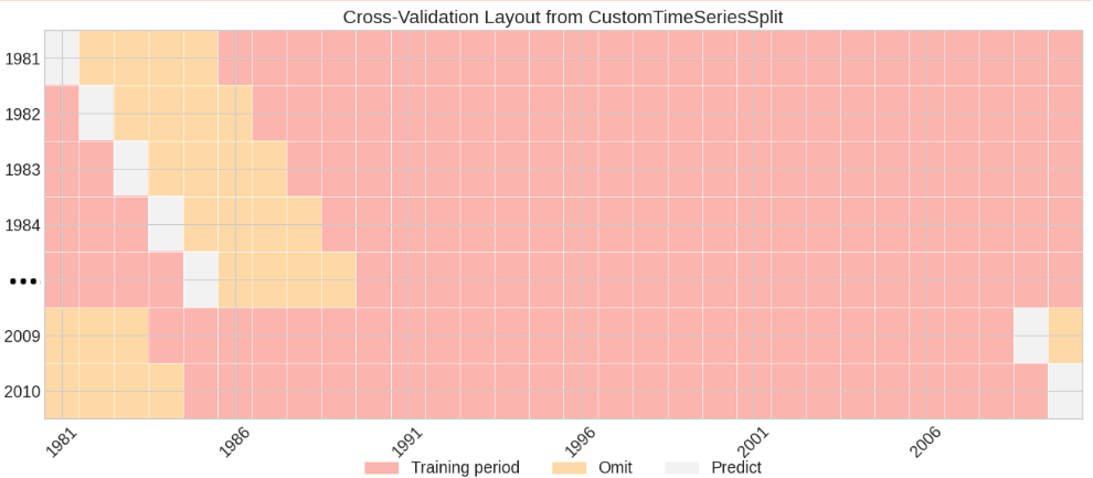
Cross-validation scheme used in wass2s
The figure shows how we split our data (1981-2010) to validate the model. Each row is a “fold” or a test run.
Pink (Training): Years we use to train the model. For example, in the first row, we train on 1986-2010.
Yellow (Omit): A buffer years we skip to avoid cheating. Climate data has patterns over time, so we don’t want to train on a years right after/before the one we’re predicting, which would make the model look better than it really is. In this case we’ve omitted four years (in the first row, we skip 1982-1985).
White (Predict): The year we predict. In the first row, we predict 1981.
CustomTimeSeriesSplit
A custom splitter for time series data that accounts for temporal dependencies.
Initialization
n_splits: Number of splits for cross-validation.
Methods
split: Generates indices for training and test sets, omitting a specified number of samples after the test index.
get_n_splits: Returns the number of splits.
WAS_Cross_Validator
A wrapper class that uses the custom splitter to perform cross-validation with various models.
Initialization
n_splits: Number of splits for cross-validation.
nb_omit: Number of samples to omit from training after the test index.
Methods
get_model_params: Retrieves parameters for the model’s compute_model method.
cross_validate: Performs cross-validation and computes deterministic hindcast and tercile probabilities.
Example Usage
from wass2s.was_cross_validate import WAS_Cross_Validator

# Initialize the cross-validator
cv = WAS_Cross_Validator(n_splits=30, nb_omit=4)
A better example will be provided in the next sections.
Estimating Prediction Uncertainty
The cross-validation makes out-of-sample predictions for each fold’s prediction period, and errors are calculated by comparing predictions to actual values. These errors are collected across all folds.
Running the statistical models—e.g. multiple linear regression—yields the most likely value of the predictand (best-guess) for the coming season.
Because seasonal outlooks are inherently probabilistic, we must go beyond this single best-guess and quantify the likelihood of other possible outcomes.
wass2s does so by analysing the cross-validation errors described earlier. The method explicitly takes the statistical distribution of the predictand into account.
If, for instance, the predictand is approximately Gaussian, we assume the predicted values follow a normal distribution whose mean is the single best-guess and whose variance equals the cross-validated error variance.
Comparing that forecast probability-density function with the climatological density (see the example in Figure 2) lets us integrate the areas that fall below-normal (values below the 1st tercile), near-normal (values between the 1st and 3rd terciles), and above-normal (values above the 3rd tercile).
These integrals are the tercile probabilities ultimately delivered to users.
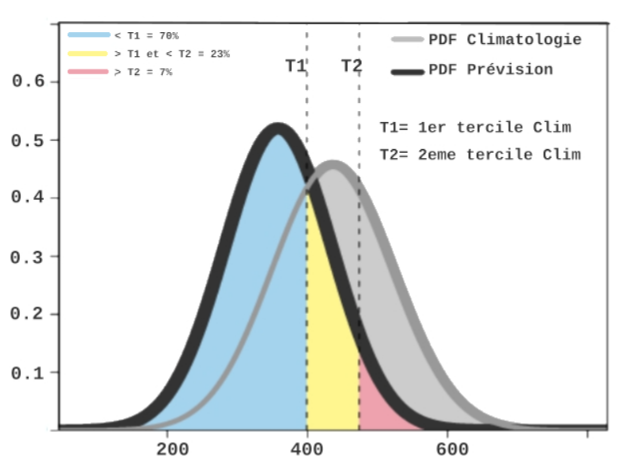
Figure 2: Generation of probabilistic forecasts
Important
Classification-based statistical models—such as logistic regression, extended logistic regression and support vector classification—do not generate continuous probabilistic forecasts over a full distribution of outcomes as indicated above. Instead, they classify the predictand into discrete categories based on climatological terciles (below-normal, near-normal, above-normal) and estimate the probability associated with each class.