Quantifying uncertainty via cross-validation
Cross-validation schemes are used to assess model performance and to quantify uncertainty. wass2s uses a cross-validation scheme that splits the data into training, omit, and test periods. The scheme is a variation of the K-Fold cross-validation scheme, but it is tailored for time series data throughout CustomTimeSeriesSplit and WAS_Cross_Validator class. The scheme is illustrated in the figure below (Figure 1).
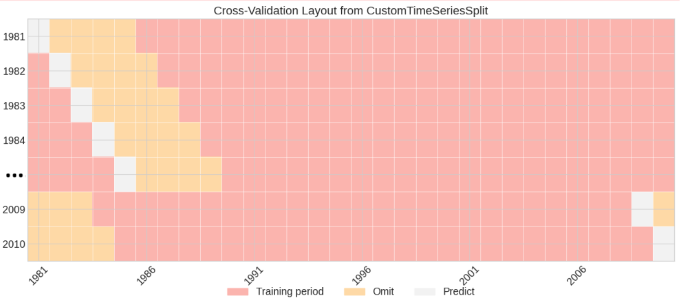
Cross-validation scheme used in wass2s
The figure shows how we split our data (1981–2010) to validate the model. Each row is a “fold” or a test run.
Pink (Training): Years we use to train the model. For example, in the first row, we train on 1986–2010.
Yellow (Omit): A buffer years we skip to avoid cheating. Climate data has patterns over time, so we don’t want to train on a years right after/before the one we’re predicting, which would make the model look better than it really is. In this case we’ve omitted four years (in the first row, we skip 1982-1985).
White (Predict): The year we predict. In the first row, we predict 1981.
CustomTimeSeriesSplit
A custom splitter for time series data that accounts for temporal dependencies.
Initialization
n_splits: Number of splits for cross-validation.
Methods
split: Generates indices for training and test sets, omitting a specified number of samples after the test index.
get_n_splits: Returns the number of splits.
WAS_Cross_Validator
A wrapper class that uses the custom splitter to perform cross-validation with various models.
Initialization
n_splits: Number of splits for cross-validation.
nb_omit: Number of samples to omit from training after the test index.
Methods
get_model_params: Retrieves parameters for the model’s compute_model method.
cross_validate: Performs cross-validation and computes deterministic hindcast and tercile probabilities.
Example Usage
from wass2s.was_cross_validate import WAS_Cross_Validator

# Initialize the cross-validator
cv = WAS_Cross_Validator(n_splits=30, nb_omit=4)
A better example will be provided in the next sections.
Estimating Prediction Uncertainty
The cross-validation makes out-of-sample predictions for each fold’s prediction period, and errors are calculated by comparing predictions to actual values. These errors are collected across all folds. Running the statistical models—e.g. multiple linear regression—yields the most likely value of the predictand (best-guess) for the coming season. Because seasonal outlooks are inherently probabilistic, we must go beyond this single best-guess and quantify the likelihood of other possible outcomes. wass2s does so by analysing the cross-validation errors described earlier. The method explicitly takes the statistical distribution of the predictand into account. If, for instance, the predictand is approximately Gaussian, we assume the predicted values follow a normal distribution whose mean is the single best-guess and whose variance equals the cross-validated error variance. Comparing that forecast probability-density function with the climatological density (see the example in Figure 2) lets us integrate the areas that fall below-normal (values below the 1st tercile), near-normal (values between the 1st and 3rd terciles), and above-normal (values above the 3rd tercile). These integrals are the tercile probabilities ultimately delivered to users.
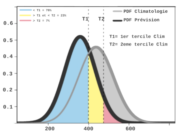
Figure 2: Generation of probabilistic forecasts
Important
Classification-based statistical models—such as logistic regression, extended logistic regression, and support vector classification—do not generate continuous probabilistic forecasts over a full distribution of outcomes as indicated above. Instead, they classify the predictand into discrete categories based on climatological terciles (below-normal, near-normal, above-normal) and estimate the probability associated with each class.